Tutorials

Discrete Markov chains

Initializing a Markov chain using some data.

>>> import mchmm as mc
>>> a = mc.MarkovChain().from_data('AABCABCBAAAACBCBACBABCABCBACBACBABABCBACBBCBBCBCBCBACBABABCBCBAAACABABCBBCBCBCBCBCBAABCBBCBCBCCCBABCBCBBABCBABCABCCABABCBABC')

Now, we can look at the observed transition frequency matrix:

>>> a.observed_matrix
array([[ 7., 18.,  7.],
       [19.,  5., 29.],
       [ 5., 30.,  3.]])

And the observed transition probability matrix:

>>> a.observed_p_matrix
array([[0.21875   , 0.5625    , 0.21875   ],
       [0.35849057, 0.09433962, 0.54716981],
       [0.13157895, 0.78947368, 0.07894737]])

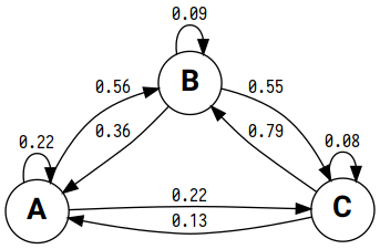
You can visualize your Markov chain. First, build a directed graph with graph_make() method of MarkovChain object. Then render() it.

>>> graph = a.graph_make(
      format="png",
      graph_attr=[("rankdir", "LR")],
      node_attr=[("fontname", "Roboto bold"), ("fontsize", "20")],
      edge_attr=[("fontname", "Iosevka"), ("fontsize", "12")]
    )
>>> graph.render()

Here is the result:

Pandas can help us annotate columns and rows:

>>> import pandas as pd
>>> pd.DataFrame(a.observed_matrix, index=a.states, columns=a.states, dtype=int)
    A   B   C
A   7  18   7
B  19   5  29
C   5  30   3

Viewing the expected transition frequency matrix:

>>> a.expected_matrix
array([[ 8.06504065, 13.78861789, 10.14634146],
       [13.35772358, 22.83739837, 16.80487805],
       [ 9.57723577, 16.37398374, 12.04878049]])

Calculating Nth order transition probability matrix:

>>> a.n_order_matrix(a.observed_p_matrix, order=2)
array([[0.2782854 , 0.34881028, 0.37290432],
       [0.1842357 , 0.64252707, 0.17323722],
       [0.32218957, 0.21081868, 0.46699175]])

Carrying out a chi-squared test:

>>> a.chisquare(a.observed_matrix, a.expected_matrix, axis=None)
Power_divergenceResult(statistic=47.89038802624337, pvalue=1.0367838347591701e-07)

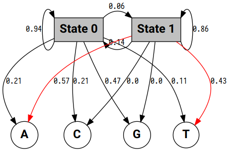
Finally, let’s simulate a Markov chain given our data.

>>> ids, states = a.simulate(10, start='A', seed=np.random.randint(0, 10, 10))
>>> ids
array([0, 2, 1, 0, 2, 1, 0, 2, 1, 0])
>>> states
array(['A', 'C', 'B', 'A', 'C', 'B', 'A', 'C', 'B', 'A'], dtype='<U1')
>>> "".join(states)
'ACBACBACBA'

Hidden Markov models

We will use a fragment of DNA sequence with TATA box as an example. Initializing a hidden Markov model with sequences of observations and states:

>>> import mchmm as mc
>>> obs_seq = 'AGACTGCATATATAAGGGGCAGGCTG'
>>> sts_seq = '00000000111111100000000000'
>>> a = mc.HiddenMarkovModel().from_seq(obs_seq, sts_seq)

Unique states and observations are automatically inferred:

>>> a.states
['0' '1']
>>> a.observations
['A' 'C' 'G' 'T']

The transition probability matrix for all states can be accessed using tp attribute:

>>> a.tp
[[0.94444444 0.05555556]
 [0.14285714 0.85714286]]

There is also ep attribute for the emission probability matrix for all states and observations.

>>> a.ep
[[0.21052632 0.21052632 0.47368421 0.10526316]
 [0.57142857 0.         0.         0.42857143]]

Converting the emission matrix to Pandas DataFrame:

>>> import pandas as pd
>>> pd.DataFrame(a.ep, index=a.states, columns=a.observations)
          A         C         G         T
0  0.210526  0.210526  0.473684  0.105263
1  0.571429  0.000000  0.000000  0.428571

Directed graph of the hidden Markov model:

Graph can be visualized using graph_make method of HiddenMarkovModel object:

>>> graph = a.graph_make(
      format="png",
      graph_attr=[("rankdir", "LR"), ("ranksep", "1"), ("rank", "same")]
    )
>>> graph.render()

Viterbi algorithm

Running Viterbi algorithm on new observations.

>>> new_obs = "GGCATTGGGCTATAAGAGGAGCTTG"
>>> vs, vsi = a.viterbi(new_obs)
>>> # states sequence
>>> print("VI", "".join(vs))
>>> # observations
>>> print("NO", new_obs)

VI 0000000001111100000000000
NO GGCATTGGGCTATAAGAGGAGCTTG

Baum-Welch algorithm

Using Baum-Welch algorithm to infer the parameters of a Hidden Markov model:

>>> obs_seq = 'AGACTGCATATATAAGGGGCAGGCTG'
>>> a = hmm.HiddenMarkovModel().from_baum_welch(obs_seq, states=['0', '1'])
>>> # training log: KL divergence values for all iterations
>>> a.log

{
  'tp': [0.008646969455670256, 0.0012397829805491124, 0.0003950986109761759],
  'ep': [0.09078874423746826, 0.0022734816599056084, 0.0010118204023946836],
  'pi': [0.009030829793043593, 0.016658391248503462, 0.0038894983546756065]
}

The inferred transition (tp), emission (ep) probability matrices and initial state distribution (pi) can be accessed as shown:

>>> a.ep, a.tp, a.pi

This model can be decoded using Viterbi algorithm:

>>> new_obs = "GGCATTGGGCTATAAGAGGAGCTTG"
>>> vs, vsi = a.viterbi(new_obs)
>>> print("VI", "".join(vs))
>>> print("NO", new_obs)

VI 0011100001111100000001100
NO GGCATTGGGCTATAAGAGGAGCTTG